The State of the Art in Biological Image Analysis
I. INTRODUCTION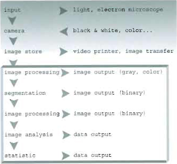 |
| FIGURE 1 Chain of image acquisition and treatment. |
The general chain of image acquisition and treatment can be sketched as shown in Fig. 1. Before undertaking analysis of a collected set of images, one should identify the most suitable procedure to be followed. In particular, two different approaches can be outlined:
- An image processing procedure (whose output is an image) requiring the use and development of tools for image enhancement.
- An image analysis procedure in which further quantitative statistics of both morphological and fluorescence intensity parameters are determined, leading to numerical data output.
II. IMAGE PROCESSING
The first steps to be performed are noise reduction, shading correction, contrast, and edge enhancement. Depending on the noise sources and the hardware devices involved, images can be processed via software or hardware. Different standard image processing routines can be run and eventually adapted according to the kind of captured and stored data input (RGB, grey scale, or binary color space, multilayered or single-layered, compressed or uncompressed).
For software data treatment, special algorithms (filters) are used or developed, either directly acting on the original numerical matrix (representative of the image) or within the frequency domain obtained by a particular mapping of the spatial data set through the Fourier transform (Diaspro et al., 2002). Although automated software with a wide range of standard and optimised filters is available, the use of these tools as black boxes can cause new unexpected artefacts to be added to images. This can be particularly risky when dealing with biological samples whose degree of complexity may often prevent the user from relying on his common sense. The final goal of these procedures is that of improving the signal to noise ratio (SNR), leading to better image visualisation without any loss of intrinsic amount of information.
III. IMAGE ANALYSIS
Quantitative image analysis deals with both collecting information from fluorescence intensity signals and obtaining morphological-geometrical parameters from the sample. Different biological treatments and data acquisition procedures (using specific off-line processing) are typically required, according to the topic under study. It is worth listing some of the most commonly used procedures: colocalization, morphological analysis [geometrical parameter estimation on threedimensional (3D) and two-dimensional (2D) samples], image classification (fractal analysis and feature extraction), and frequency domain analysis (Diaspro et al., 1990; Castleman, 1996).
IV. COLOCALIZATION
The observations of in vivo cellular details and events often involve the use of single or multifluorescence labelling with a high degree of specificity with the respect of the structures under investigation. The necessity of simultaneously imaging different functional parts of samples (such as microtubules, nuclei or mitochondria) demands the use of multiple distinct fluorescence dyes in order to reveal the parts of interest by keeping them visually distinct from one another. In this situation, image acquisition is typically carried on separately at the different excitation wavelengths and the later offiine analysis may deal, among other things, with one more problem: that of extracting information about the eventual overlap (colocalization) between the different fluorescence signals expressed by the various part of the sample, which thus occupy the same physical location. This is a crucial task, especially in biological and medical studies where one is interested in studying the molecules distribution with the respect of particular functional structures such as receptors.
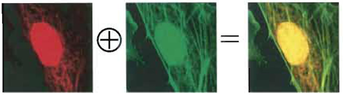 |
| FIGURE 2 Two-photon imaging (750-nm wavelength) of an artery endothelial bovine pulmonary cell. Mitochondria (labelled with MitoTracker) are visible in the red channel, actin filaments (labelled with BODIPY) in the green one, and nuclei (labelled with DAPI) in both. The emission intensity of the nucleus is much higher than the others due to the strong concentration of DNA-bounded DAPI inside the cell with respect to the other dyes. Colocalized pixels are yellow ones in the RGB image (Diaspro, 2001). |
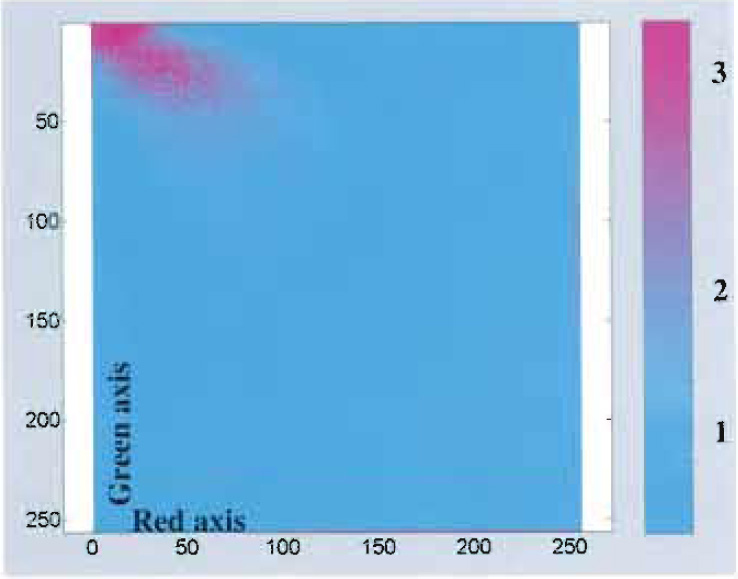 |
| FIGURE 3 Scatter plot: purple dots represent highly colocalized red-green intensity pixels. |
In addition to this visualisation, a proper quantification of the degree of colocalization can be obtained by comparing each of the acquired images by means of suitable coefficients (Fig. 4), which may account either for the similarity of shapes between the two images (without considering intensities) or for the difference of intensity between colocalized pixels, depending on the kind of information one is interested in.
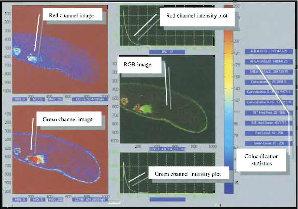 |
| FIGURE 4 Snapshot of a typical image analysis user interface for colocalization analysis. Courtesy of Marco Raimondo and Paola Ramoino, LAMBS, http://www.lambs.it. |
A. Morphological Analysis and Classification
Morphological investigations of images are strictly connected to the idea of topological space due to the mathematical environment wherein tools for quantitative analysis are developed. As a first step, this requires a unequivocal relationship between each image array and a set of real space coordinates to be established. For single-layered images, this goal can be accomplished by dividing the field of view (i.e., the real dimension of the region within the image) by the number of pixels, thus getting the effective size of the elementary dot in the image. This is all one typically needs for geometrical calculations in the plane. Multilayered images naturally involve a third dimension so that one more relationship needs to be established between the optical sections and their real world distance from one another. The simplest approach for solving this task consists of assigning the optical sectioning distance (eventually scaled to account for further data acquisition artefacts) to two contiguous slices. Once these correspondences are established between the images and the topological space, further and more complex computer- based processing can be performed, including 3D sample reconstruction (Fig. 5), morphometrical estimations, object counting, and localization (Bianco and Diaspro, 1989; Diaspro et al., 1990).
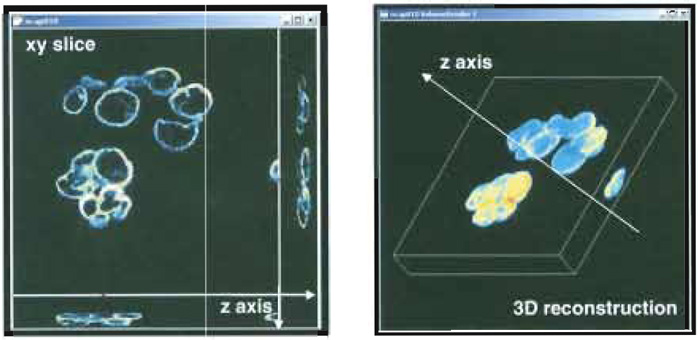 |
| FIGURE 5 Snapshot of a 3D sample data acquisition (left) and 3D sample reconstruction (right). |
The need of morphometrical measurements is often the main prerequisite in most biological and medical comparative studies where the shape and dimension of structural components of the samples (such as tissues, cells, and organlets) are strictly related to their functions. In these cases, an effective 3D visualization may be nice looking while failing to provide accurate results in terms of accurate characterization of the structural properties of interest. It is far better to use suitable stereological methods, implemented using highly efficient software, involving single slices. These procedures can be either semi-interactive or completely automated. The main difference between these two approaches is that the latter ones are faster but require reliable automatic thresholding and segmentation routines for the recognition of the objects of interest within the images.
Several different stereological methods have been tested and improved over the years: the optical dissector principle (Gundersen, 1986; Sterio, 1984) or the unbiased sampling brick rule (Howard et al., 1985) for particles counting; the nucleator (Gundersen, 1988) and the planar rotator (Jensen and Gundersen, 1993) applied to a stack of optical sections for estimating the mean particle volume; the optical rotator (Kieu and Jensen, 1993; Tandrup et al., 1997), spatial grid method (Sandau, 1987), and "Fakir method" (Kubinova and Janacek, 1998) for surface area estimation; and the vertical slices method (Gokhale, 1990) and global spatial sampling (Larsen et al., 1998) for length estimation. Moreover, volume and surface area or curve length estimation can be obtained with known precision and are considered to be free from any systematic error (bias) relating to the sample strategy. Furthermore, they can be undertaken without any previous assumptions about the shape or the structure of the objects under investigation, thus allowing the user to get a realistic average value of the parameters of interest as a result of an average obtained from repeated measurement processes. One more important parameter for many computer vision tasks, such as image classification, is texture segmentation, consisting of splitting an image into regions of similar texture. This task is usually performed in two stages: texture feature extraction (to characterize each texture) and further texture segmentation (to determine homogeneous regions), allowing a proper segmentation of the image.
The limiting factors for all these investigations are the resolution of the imaging system, determined by its point spread function (PSF), and the intrinsic reproducibility of the observed phenomenon itself, which if poor might demand an improvement in the accuracy of the data acquisition protocol (Bianco and Diaspro, 1989; Castleman, 1996).
The approaches discussed so far mainly rest on some common properties of the familiar topological space, but there exist in nature objects whose properties are not fully analysable by any possible set of standard topological parameters. When considering the morphology of samples, for instance, it is very common to take into account those geometrical parameters suggested by a suitable modelling of structures, involving elementary shapes such as lines, circles, spheres, or simple polygon. This allows one both to obtain a preliminary quantitative analysis of the geometrical properties of the samples and to cluster them according to the values of some characteristic parameters. Unfortunately, this method cannot always be applied successfully, as most of the complex biological structures cannot be modelled easily by simple shapes. One popular example is that of the branching structure of many biological structures, such as the arteries, veins, nerves, the parotid gland ducts, or the bronchial tree in the human body. The presence of a certain selfsimilarity and the lack of a well-defined scale suggest that a complete characterization cannot be based simply on a conventional surface/volume estimation, as such a numerical value does not convey any further information about the degree of complexity of the shape to which it is related. These empirical evidences lead to the idea that some other independent parameter might exist, something like a space-filling factor: this is the fractal dimension (fd), existing somewhere between the usual topological dimensions, whose value ranges between 1 and 2, respectively, depending on whether the object fills almost no space (such as in the case of a line) or fills all the available space (such as in the case of a square or a circle). A combination of fractal dimension and standard texture features has been shown to provide better discrimination than standard texture features alone. An example of this application is that related to the study of the breaking strength of bones. Despite the fact that there is a strong dependence of breaking strength on mineral density, more refined models are required to explain variations in the strength of bones having identical densities. Consideration of the way in which mineral density is arranged within the bones, thus influencing their structural resistance, has led to the use of the fractal index as a parameter, which is both calculated easily from images and particularly efficient for their classification. Other studies employing fractal analysis have involved the characterization of mammographic patterns (Caldwell et al., 1990), colorectal polyps (Cross et al., 1994), trabecular bones (Cross et al., 1993a; Majumdar et al., 1993; Benhamou et al., 1994), retinal vessels (Mainster, 1990), renal arteries (Cross et al., 1993b), Papanicolaou-stained cervical samples (MacAulay et al., 1990), and epithelial lesions (Landini et al., 1990).
It is worth pointing out here that a variety of procedures have been proposed for estimating the fd of images, such as the box-counting method (BC) or the fractional Brownian motion method (FBM); the best algorithm for the job will vary according to the kind of images under study. It can be shown that the BC method is ineffective if applied to low-resolution images, whereas the FBM one reveals its limits when applied to noisy images or to systems with strong local scaling factors.
Moreover, because every fd calculation needs a threshold level to be set in order to discriminate different regions within the same image, this implies the existence of a fractal spectrum in which the value of fd depends on the threshold level. The best choice for this threshold can be made either from prior knowledge about the inner structure of the sample or through some parameters (such as the linear correlation coefficient for the BC method), intrinsic to the particular fd algorithm used, which may somehow account for the fractal dimension.
B. Frequency Domain
Some image analysis techniques employed in a wide range of applications, such as image filtering, reconstruction and compression, turn time domain inputs into frequency domain outputs. A representation of a given multidimensional signal in the frequency domain is often useful for identifying periodical components within signals.
The Fourier transform provides a unique and invertible mapping of original data to frequency domain data represented as complex numbers, termed structure factors, in which the frequency characteristics are displayed in terms of their magnitudes and phases. Both the magnitude and the phase functions of the structure factors are necessary for the complete reconstruction of an image from its Fourier transform. The magnitude-only image is unrecognizable and has severe dynamic range problems. The phase-only image is barely recognizable, i.e., severely degraded in quality. The advantage of using the Fourier transform lies in its invariant properties. It is easy to demonstrate, for instance, that rotating the object merely causes a phase change to occur and that the same phase change is caused to all the structure factors. The magnitude is independent of the phase and so is unaffected by rotation. (This is an example of the very important property of shift invariance.) Second, consider a change of size of the object. This does not change any of the phases and changes the magnitudes of all the structure factors by the same factor. If the magnitude of the spectrum is normalised, then it is invariant to object size as well. Finally, consider the effect of noise and quantisation errors on the boundary. This will cause local variation of high frequency components and will not change the low frequencies. Hence, if the high frequency components of the spectrum are ignored, the rest of the spectrum is unaffected by noise. Thus, for object recognition, the Fourier descriptor offers many advantages and is very useful not only in comprehensively understanding digital image analysis, but also in digital image processing. It could be a useful tool to deal with texture analysis, which is an important field in remote sensing, and it is fast to compute.
V. CONCLUSIONS
This article outlined the fundamental concepts of image processing and image analysis, addressing the main methods and giving a full list of references for deeper insights on topics of interest.
References
Benhamou, C. L., Lespessailles, E., Jacquet, G., Harba, R., Jennane, R., Loussot, T., Tourliere, D., and Ohley, W. (1994). Fractal Organization of Trabecular Bone Images on Calcaneus Radiographs. J Bone Min. Res. 9, 1909-1918.
Bianco, B., and Diaspro, A. (1989). Analysis of three-dimensional cell imaging obtained with optical microscopy techniques based on defocusing. Cell Biophys. 15(3), 189-199.
Caldwell, C. B., Stapleton, S. J., Holdsworth, D. W., Jong, R. A., Weiser, W. J., Cooke, G., and Yaffe, M. J. (1990). Characterisation of mammographic parenchymal pattern by fractal dimension. Phys. Med. Biol. 35, 235-247.
Castleman, K. R. (1996)."Digital Image Processing." Prentice Hall, Englewood Cliffs, NJ.
Cross, S. S., Bury, J. P., Silcocks, P. B., Stephenson, T. J., and Cotton, D. W. K. (1994). Fractal geometric analysis of colorectal polyps. J. Pathol. 172, 317-323.
Cross, S. S., et al. (1993a). Trabecular bone does not have a fractal structure on light microscopic examination. J. Pathol. 170, 311-313.
Cross, S. S., Start, R. D., Silcocks, P. B., Bull, A. D., Cotton, D. W. K., and Underwood, J. C. E. (1993b). Quantitation of the renal arterial tree by fractal analysis. J. Pathol. 170, 479-484.
Diaspro, A. (ed.) (2002). "Confocal and Two-photon Microscopy: Foundations, Applications and Advances." Wiley-Liss, New York.
Diaspro, A., Adami, M., Sartore, M., and Nicolini, C. (1990). IMAGO: A complete system for acquisition, processing, two/threedimensional and temporal display of microscopic bio-images. Comput. Methods Programs Biomed. 31(3-4), 225-236.
Gokhale, A. M. (1990). Unbiased estimation of curve length in 3D using vertical slices. J. Microsc. 159, 133-141.
Gundersen, H. J. G. (1986). Stereology of arbitrary particles: A review of unbiased number and size estimators and the presentation of some new ones, in memory of William R. Thompson. J. Microsc. 143, 3-45.
Gundersen, H. J. G. (1988). The nucleator. J. Microsc. 151, 3-21.
Howard, C. V., Reid, S., Baddeley, A., and Boyde, A. (1985). Unbiased estimation of particle density in the tandem scanning reflected light microscope. J. Microsc. 138, 203-212.
Kieu, K., and Jensen, E. B. V. (1993). Stereological estimation based on isotropic slices through fixed points. J. Microsc. 170, 45-51.
Kubinova, L., and Janacek, J. (1998). Estimating surface area by isotropic fakir method from thick slices cut in arbitrary direction. J. Microsc. 191, 201-211.
Jensen, E. B. V., and Gundersen, H. J. G. (1993). The rotator. J. Microsc. 170, 35-44.
Landini, G., and Rippin, J. W. (1993). Fractal dimensions of the epithelial-connective tissue interfaces in premalignant and malignant epithelial lesions of the floor of the mouth. Anal. Quant. Cyt. Hist. 15, 144-149.
Larsen, J. O., Gundersen, H. J. G., and Nielsen, J. (1998). Global spatial sampling with isotropic virtual planes: Estimators of length density and total length in thick, arbitrarily orientated sections. J. Microsc. 191, 238-248.
MacAulay, C., and Palcic (1990). Fractal texture features based on optical density surface area. Anal. Quant. Cyt. Hist. 12, 394-398.
Mainster, M. A. (1990). The fractal properties of retinal vessels: Embryological and clinical implications. Eye 4, 235-241.
Majumdar, S., Weinstein, R. S., and Prasad, R. R. (1993). Application of fractal geometry techniques to the study of trabecular bone. Med. Phys. 20, 1611-1619.
Manders, E. M. M., Verbeek, F. J., and Aten, J. A. (1993). Measurement of co-localization of objects in dualcolor confocal images. J. Microsc. 169, 375-382.
Puig, D., and Garcfa, M. A. (2001). Determining optimal window size for texture feature extraction methods. In "IX Spanish Symposium on Pattern Recognition and Image Analysis," Vol. 2, pp. 237-242.
Robert, N., Puddephat, M. J., and McNulty, V. (2000). The benefit of stereology for quantitative radiology. Br. J. Radiol. 73, 679-697.
Sandau, K. (1987). How to estimate the area of a surface using a spatial grid. Acta Stereol. 6, 31-36.
Sterio, D. C. (1984). The unbiased estimation of number and sizes of arbitrary particles using the disector. J. Microsc. 134, 127-136.
Tamames, J., Clark, D., Herrero, J., Dopazo, J., Blaschke, C., Fernandez, J. M., Oliveros, J. C., and Valencia, A. (2002). Bioinformatics methods for the analysis of expression arrays: Data clustering and information extraction. J. Biotechnol. 98, 269-283.
Tandrup, T., Gundersen, H. J. G., and Jensen, E. B. V. (1997). The optical rotator. J. Microsc. 186, 108-120.
Support our developers